5.1 Daily download of R-packages
Finding 1: There was unusual download activity in one day of 2014 and 2018.
In this first section, we studied the daily downloads of CRAN R-packages from 2012-10-01 to 2021-06-07. The data was obtained from the cranlogs package(Csárdi 2019), which includes a summary of the download logs from the RStudio CRAN mirror. The daily download data for CRAN R-packages are available from 1st October 2012. Examination of this data showed two unusual observations in 2014 and 2018 as shown in Figure 5.1. The one happening in 2014 was on 2014-11-17, which was Monday, while the other one happening in 2018 was on 2018-10-21, which was on Sunday.
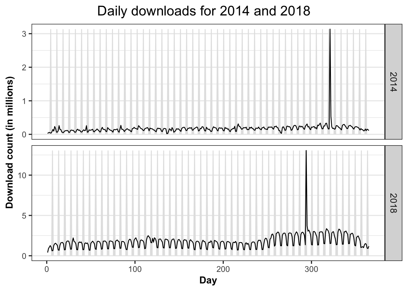
Figure 5.1: Unusual download spikes on 2014 and 2018.
Then let’s have a closer look into these two spikes. First, we focused on the spike on 2014-11-17. From Table 5.1, we could see that the downloads of top downloaded R-packages on this day differs little, so it’s not due to certain package.
| package | n |
|---|---|
| BayHaz | 767035 |
| clhs | 660298 |
| GPseq | 394840 |
| OPI | 382518 |
| YaleToolkit | 370513 |
| survsim | 224994 |
| BAT | 40592 |
| Rcpp | 3509 |
| ggplot2 | 3167 |
| plyr | 3150 |
Table 5.2 shows the downloads from different countries. It is obvious that downloads from Indonesia is much more than any others, which indicates the most downloads are from Indonesia.
| country | n |
|---|---|
| ID | 2863576 |
| US | 96336 |
| CN | 32729 |
| DE | 14548 |
| FR | 11860 |
| GB | 10491 |
| IN | 8635 |
| HK | 8090 |
| BE | 7720 |
| KR | 6794 |
Furthermore, we also checked the IP address in Table 5.3, downloads from ip3758 is much higher than others. So, it seems that most of the downloads are owing to one certain IP.
| ip_id | n |
|---|---|
| 3758 | 2863432 |
| 11536 | 6244 |
| 11725 | 5992 |
| 16385 | 5991 |
| 534 | 5986 |
| 3784 | 5983 |
| 18519 | 4511 |
| 80 | 2124 |
| 27 | 1892 |
| 464 | 1375 |
Next, let’s turn to the one in 2018. Table 5.4 shows the downloads from tidyverse is much higher than others with nearly three orders of magnitude.
| package | n |
|---|---|
| tidyverse | 11692582 |
| Rcpp | 16263 |
| stringi | 13981 |
| rlang | 13796 |
| ggplot2 | 13306 |
| dplyr | 13081 |
| glue | 12593 |
| digest | 12302 |
| stringr | 11505 |
| fansi | 11275 |
As for the country, from Table 5.5 we could know that US is much higher than any other country.
| country | n |
|---|---|
| US | 12140853 |
| NA | 179847 |
| GB | 76624 |
| IN | 51502 |
| CN | 46095 |
| TR | 36590 |
| AU | 35078 |
| DE | 32837 |
| CA | 31125 |
| KR | 30469 |
Finally, the most interesting finding is in IP address displayed in Table 5.6. Several consecutive IPs have highly distinguished downloads. It seems that they are from same person, or it is also probably a server test issue in the same short period of time.
| ip_id | n |
|---|---|
| 266 | 3034720 |
| 263 | 2457383 |
| 655 | 2099321 |
| 264 | 1557640 |
| 267 | 1406876 |
| 265 | 1032535 |
| 2 | 179711 |
| 268 | 99932 |
| 112 | 34397 |
| 3296 | 17223 |
To sum up, we found that these two unusual spikes have one thing in common, that is, most of the downloads came from a specific country. The difference is that in 2014, a large number of downloads came from several different R-packages, while in 2018, they came from only one package tidyverse. In addition, in 2014, a large number of downloads came from one IP, while in 2018, they came from several consecutive IPs, At this point, we guess it should come from the same person, and it is likely to be sever test issue, for it may be not necessary or reasonable for an individual to generate such a large quantities of downloads in one day.
Finding 2: There is an increasing number of downloads over time. This likely attests to the growing number of R users.
Figure 5.2 shows the download trend of all R-packages on CRAN over time after fixing the unusual spikes. It shows an upward trend over time, and the variance also increases with the download count, which means the volatility of the data is increasing.
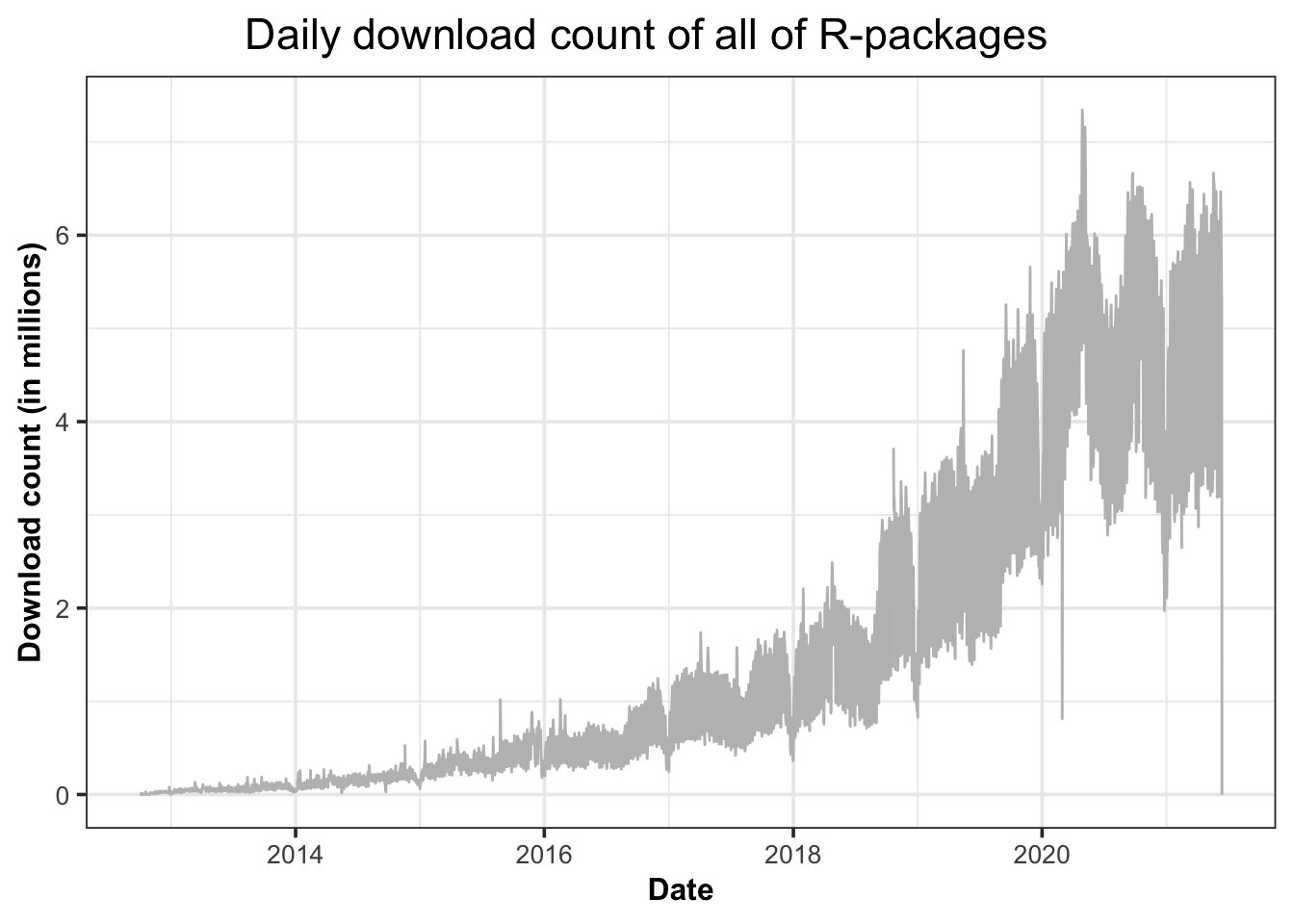
Figure 5.2: The download trend of all R-packages on CRAN over time.
Finding 3: Weekends have a lower download than weekdays.
To have a closer look at the weekly pattern, figure 5.3 shows the daily downloads of all CRAN R-packages from the RStudio mirror with the grey areas highlighting the weekend.
To be more specific, we could know that except for 2012 and 2013, the patterns of other years are very similar, that is, they all show strong weekly seasonality. To be more detailed, in 2012, the download logs showed an overall upward trend, because more and more users began to download R-packages from CRAN after its open. In the following years, there is no obvious trend in download volume, but a strong seasonality, which indicates that in a week, the total downloads always increases first then decreases, and reaches the lowest at the weekend. Although the pattern of 2013 is more volatile, it still conforms to that. We think for 2013, that is because CRAN is only open for a short time at this time, and the amount of data downloaded is not adequate to show its download pattern very clearly. Considering this, we could see that after 2016, the pattern of each year is quite consistent, for the total download has been increasing year by year. Back to weekly seasonality, that is because people are more likely to download and use packages in weekdays, and rest on weekends. And that’s why the trough of download curve always occurs on weekends. In addition, we could also notice that the lowest downloads across the year are always at the end of December and the beginning of January, probably due to the Christmas and New Year’s holidays. What’s more, the downloads is on the rise from August to October and from February to April, which covers the start of semester for most universities.
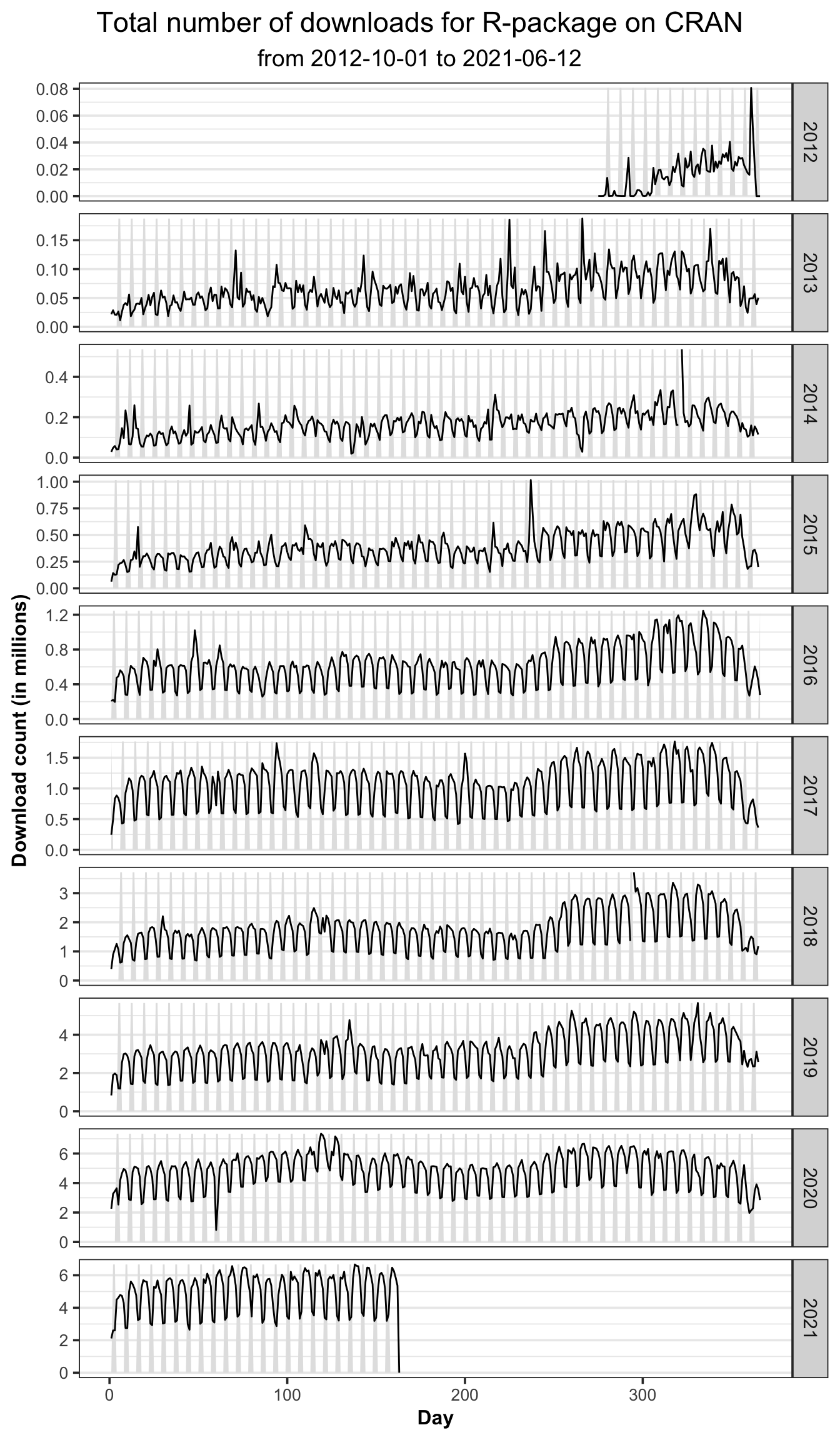
Figure 5.3: The figure shows the total downloads of all R-packages on CRAN would decrease on weekends.
As there are many fluctuation in daily download pattern which is due to calendar effect and server issue of CRAN mirror, we then applied a model called STL decomposition explained in “Forecasting: Principles and Practice (3rd Ed)” (n.d.), to smooth the curve for all the R-packages.
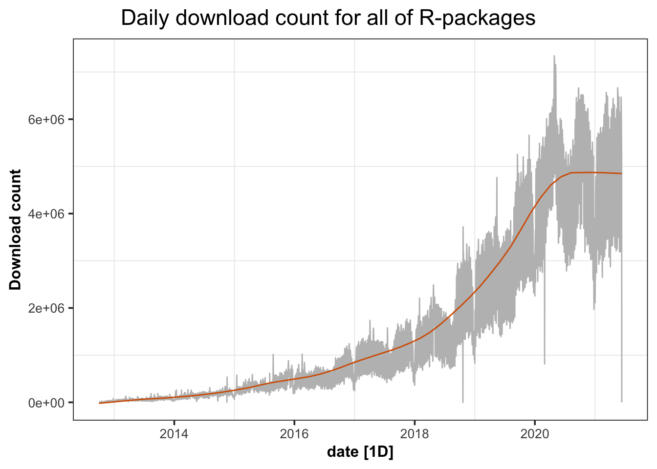
Figure 5.4: The figure shows the total downloads of all R-packages on CRAN after smoothing.
And this can be applied to any R-package to adjust the daily download pattern. In this case, we selected two packages fable and forecast as an example in Figure 5.5. It can be seen that the pattern is smoother after removing the seasonality and ignorance of extremum possibly caused by repeated downloads, updates and test downloads from the server.
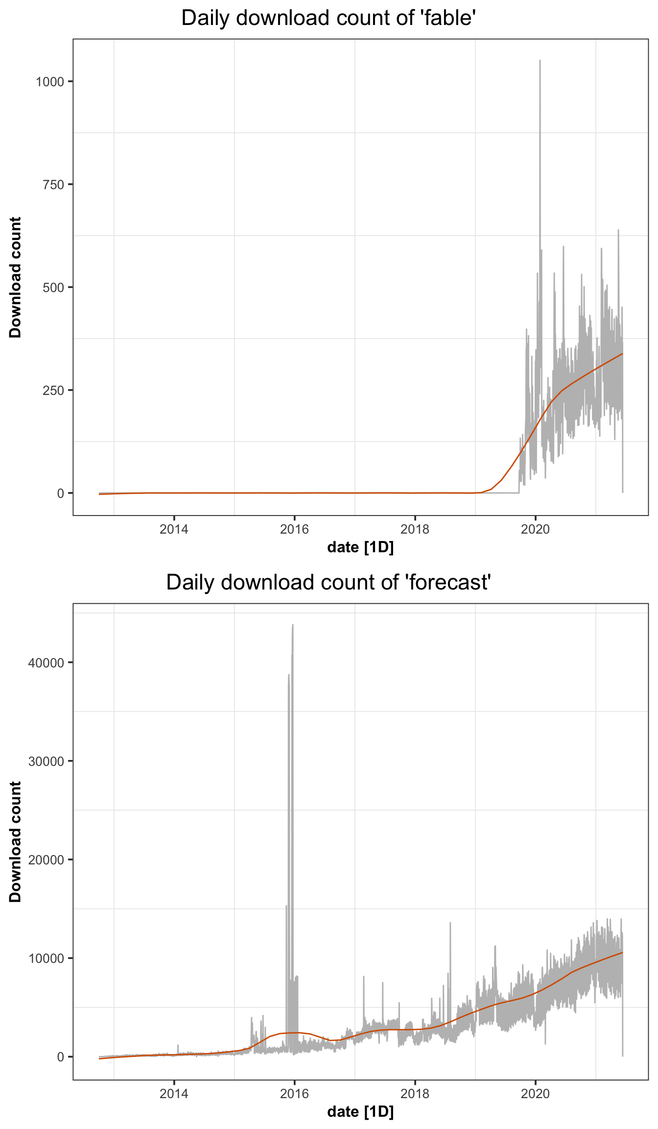
Figure 5.5: The figure shows the daily downloads of fable and forecast on CRAN after smoothing.
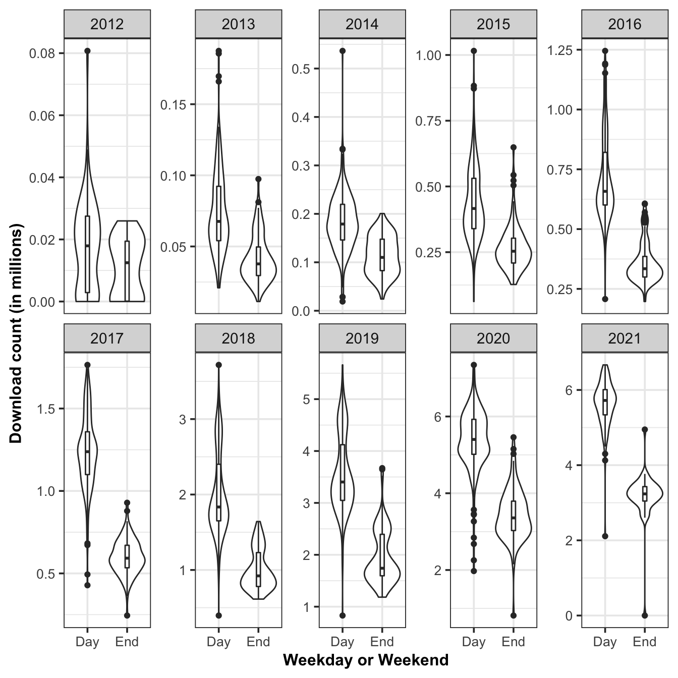
Figure ?? shows the distribution and the median of the downloads between weekday and weekends. The distribution of weekdays and weekends are quite different. Weekends are wider and shorter, while weekdays are thinner and higher, because the total download of data on weekends is less than that on weekdays. And in 2012, the median and interquartile range of download logs are not very distinguished between weekdays and weekends, for the data volume was not adequate at this time as mentioned above. But after 2013, the gap between the two becomes more and more obvious, that is, the median downloads of working days is significantly higher than that of weekends, and the overall number of data is also significantly higher than that of weekends as well. But interestingly, the lower adjacent sometimes occurs on weekends, such as in year 2014, 2015, 2018, 2019 and 2021, while sometimes in weekdays, such as in year 2012, 2013, 2016, 2017 and 2020.
Finding 4: Top 10% downloaded R-packages share nearly 90% cumulative download count of the whole.
From the previous analysis, we could see that the cumulative download count of R-packages shows an increasing trend. It would be perfect equality if every R-package had the same download count – the last 20% downloaded R-packages would gain 20% of the total download count or the top 60% downloaded R-packages would get 60% of the total download count. But we know from experience that this is obviously impossible, so here we introduced Lorenz curve(Pettinger, n.d.) to show the respective number of R-packages of different download levels (groups defined by quantiles of download count). In this way, we could figure out how many download counts contributed by different downloaded R-packages.
Figure 5.2 shows cumulative download count against each downloaded group. It can be seen that most of the download counts come from the top 10% downloaded R-packages. At the same time, we could also observe that the Gini value is close to 1, which indicates that the download volume among groups is very unbalanced. In fact, the download volume of the top 10% group is extremely distinguished from that of the following groups. It’s not hard to understand that this group should contain some R-packages with high popularity and large quantities of users. For example, if we extracted the first 10 packages of this group in Table 5.7, we could find that they are all quite famous and frequently-used ones.
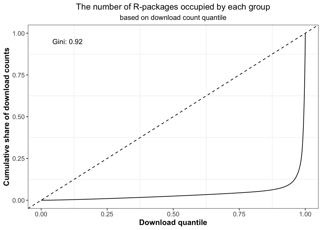
Figure 5.6: Percentiles of the download count against cumulative download count of R-packages at or below that percentile.
| package | total |
|---|---|
| rlang | 15572507 |
| vctrs | 13544857 |
| dplyr | 12739206 |
| ggplot2 | 12670952 |
| jsonlite | 12627542 |
| lifecycle | 11124212 |
| tibble | 10935860 |
| magrittr | 10312021 |
| pillar | 9566463 |
| glue | 9534999 |